Segmenting Audience with KMeans and Voronoi Diagram using Spark and MLlib

Analyzing huge data set to extract meaningful properties can be a difficult task. Several methods have been developed for the last 50 years to find hidden information.

Clustering algorithms can be used to group similar news like in Google News, find areas with high crime concentration, find trends, .. and segment the data into groups. This segmentation can be used for instance by publisher to reach a specific target audience.

In this post, we will be using the k-means clustering algorithm implemented in Spark Machine Learning Library(MLLib) to segment the dataset by geolocation .

The k-mean clustering algorithm is an unsupervised algorithm meaning that you don’t need to provide a training example for it to work(unlike neural network, SVM, Naives Bayes classifiers, …). It partitions observations into clusters in which each observation belongs to the cluster with the nearest mean. The algorithm takes as input the observations, the number of clusters(denoted k) that we want to partition the observation into and the number of iterations. It gives as a result the centers of the clusters.

The algorithm works as follow:

1. Take k random observations out of the dataset. Set the k centers of the clusters to those points
2. For each observation, find the cluster center which is the closest and assign this observation to this cluster
3. For each cluster, compute the new center by taking the average of the features of the observations assigned to this dataset
4. Go back to 2 and repeat this for a given number of iterations

The centers of the clusters will converge and will minimize the cost function which is the sum of the square distance of each observation to their assigned cluster centers.

This minimum might be a local optimum and will depend on the observation that were randomly taken at the beginning of the algorithm.

In this post, we are going to listen to a tweet stream to get tweets with their geolocation and then apply the k-means algorithm on their coordinates to find geographical clusters.

Prerequisites

In order to run our example, we need to install the followings:

• Scala 2.10+
• SBT
• simplevoronoi

To install the simplevoronoi library in your local maven repo, first download it at: http://sourceforge.net/projects/simplevoronoi/

Then uncompress the archive and install it:

tar xvfz simplevoronoi-trunk-20110706.tar.gz
cd simplevoronoi
mvn install

 

Fetching the tweets

Twitter provides an API to continuously listen to a stream of tweets. In order to use the API, you need a twitter api keys and access tokens.
To get those, log in on https://apps.twitter.com/
Click on “Create New App”. Fill in the Name, Description, Website, Callback URL and click on “Create your twitter application”.
Now go to the “API Keys” tab and click on “Create my access token”
To run the program to listen to a tweet stream and write the tweets to disk, we would need to create the file twitter-credentials.txt on your disk with the following content:

TWITTER_API_KEY=<API KEY>
TWITTER_API_SECRET=<API SECRET>
TWITTER_ACCESS_TOKEN=<ACCESS TOKEN>
TWITTER_ACCESS_TOKEN_SECRET=<ACCESS TOKEN SECRET>

Then run the program to listen to tweets:

sbt "run-main com.chimpler.example.kmeans.FetchTweets twitter-credentials.txt tweets.csv"

Wait for at least 10 minutes to get enough tweets. When you want to stop the program, just press CTRL + C.

The file tweets.csv contains lines like that:

<longitude>, <latitude>, <timestamp>, <userId>, <tweet message>

-56.544541,-29.089541,1403918487000,1706271294,Por que ni estamos jugando, son más pajeros estos locos! 😐
-69.922686,18.462675,1403918487000,2266363318,Aprenda hablar amigo
-118.565107,34.280215,1403918487000,541836358,today a boy told me I'm pretty and he loved me. he's six years old so that's good.
121.039399,14.72272,1403918487000,362868852,@Kringgelss labuyoo. Hahaha
-34.875339,-7.158832,1403918487000,285758331,@keithmeneses_ oi td bem? sdds 😔💚
103.766123,1.380696,1403918487000,121042839,Xian Lim on iShine 3 2

Alternatively, if you don’t want to create a twitter account, you can use the file tweets_small.csv containing 10,000 tweets provided in the project.

Running kmeans with spark

To run the k-means algorithm in Spark, we need to first read the csv file

  val sc = new SparkContext("local[4]", "kmeans")
  // Load and parse the data, we only extract the latitude and longitude of each line
  val data = sc.textFile(arg)
  val parsedData = data.map {
    line =>
      Vectors.dense(line.split(',').slice(0, 2).map(_.toDouble))
  }

Then we can run the spark kmeans algorithm:

  val iterationCount = 100
  val clusterCount = 10
  val model = KMeans.train(parsedData, clusterCount, iterationCount)

To determine the number of clusters, just try some values until you visually find meaningful grouping or you have a lower cost value.

The model object exhibits the following methods:

• clusterCenters: returns the centers of each cluster
• cost: returns the cost (sum of square distance of each tweets from its cluster center). The lower it is, the better.
• predict(Vector): return the cluster id closest to the vector point

From the model we can get the cluster centers and group the tweets by cluster:

  val clusterCenters = model.clusterCenters map (_.toArray)

  val cost = model.computeCost(parsedData)
  println("Cost: " + cost)

  val tweetsByGoup = data
    .map {_.split(',').slice(0, 2).map(_.toDouble)}
    .groupBy{rdd => model.predict(Vectors.dense(rdd))}
    .collect()
  sc.stop()

Note that if you run kmeans multiple times on the same data set, you can have different results as the cluster centers are initialized at random at the beginning of the algorithm.

Representing the clusters on a map

If you are not familiar with longitude, latitude coordinates, you can look at a previous post that we wrote to represent a tweet heat map on a world map.

Drawing the map background

As described in out previous post, we are using a equirectangular projection world map.

  private def drawMapBackground() {
    val mapBackground = ImageIO.read(KMeansApp.getClass.getClassLoader.getResourceAsStream(backgroundImageFileName))
    graphics.drawImage(mapBackground, 0, 0, imageWidth, imageHeight, Color.WHITE, null)
    graphics.setColor(new Color(0, 0, 0, 100))
    graphics.fillRect(0, 0, imageWidth, imageHeight)
  }

Choosing the colors

To generate a color for each cluster, we can choose colors at random but it will often give some bad results: colors too close too each other, colors too bright or too dark, …

An easy way to generate colors is to use the HSL Color Model(Hue, Saturation, Lightness). With the hue ranging from 0 to 360 going from red to yellow to green to blue and back to red with all the intermediary values in-between.

We choose a fixed value for the saturation and lightness and set the hue value based on the group number:

def generateColor(group: Int, groupCount: Int): Color = {
  val hue = group.toFloat / groupCount
  val saturation = 0.8f
  val lightness = 0.5f
  Color.getHSBColor(hue, saturation, lightness)
}

Draw tweets on the map

To translate the longitude and latitude into image coordinates, we only need to scale the coordinates and offset them depending on the image size:

  private def toImageCoordinates(longitude: Double, latitude: Double, imageWidth: Int, imageHeight: Int): (Int, Int) = {
    (
      (imageWidth * (0.5 + longitude / 360)).toInt,
      (imageHeight * (0.5 - latitude / 180)).toInt
      )
  }

We can use this method to draw the tweets on the map

  private def drawTweets() {
    for ((group, tweets) <- tweetsByGoup) {
      val color = groupColors(group).brighter()
      graphics.setColor(new Color(color.getRed, color.getGreen, color.getBlue, 50))
      for (coordinate <- tweets) {
        val (x, y) = Utils.toImageCoordinates(coordinate(0), coordinate(1), imageWidth, imageHeight)
        graphics.fillOval(x - 1, y - 1, 2, 2)
      }
    }
  }

And also draw the cluster centers

  private def drawClusterCenters() {
    for (group <- 0 until clusterCount) {
      val (x, y) = toImageCoordinates(clusterCenters(group)(0), clusterCenters(group)(1), imageWidth, imageHeight)

      // draw center circle
      val color = groupColors(group)
      graphics.setColor(color)
      graphics.fillOval(x - 6, y - 6, 12, 12)
      graphics.setColor(Color.WHITE)
      graphics.drawOval(x - 6, y - 6, 12, 12)
    }
  }

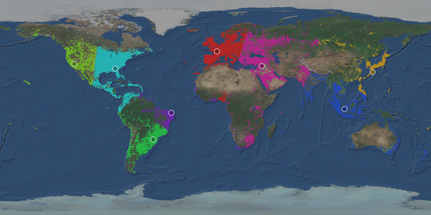
With this representation, we can see two issues: 1) It can be difficult to see the areas associated to each the cluster, 2) It’s hard to see the density of the points.
We are going to address those two issues in the next sections.

Voronoi Diagram

A Voronoi diagram is a way of dividing the space into regions. Each cluster center is associated to a region such that any points in that region is closer to this cluster center than to any other cluster centers.

One way to find Voronoi cells out of a set of points is by using the Fortune’s algorithm. It is implemented in the simplevoronoi library.

val xValuesIn = clusterCenters map (_(0))
val yValuesIn = clusterCenters map (_(1))

val voronoi = new Voronoi(0.0001)
val graphEdges = voronoi.generateVoronoi(xValuesIn, yValuesIn, -180d, 180d, -90d, 90d)

The generateVoronoi returns a list of edges with the following properties:

• x1, y1: one end of the edge
• x2, y2: the other end of the edge
• site1, site2: the two regions the edge is separating

We are going to use those information to find the polygon that surrounds each region.

First, we are going to group the edges by region:

    val edgeBySite = new Array[mutable.Buffer[GraphEdge]](clusterCount)
    for (i <- 0 until clusterCount) edgeBySite(i) = mutable.Buffer.empty[GraphEdge]

    for (edge <- graphEdges) {
      // skip edge with 0 length (bug in voronoi lib?)
      if (edge.x1 != edge.x2 || edge.y1 != edge.y2) {
        edgeBySite(edge.site1) += edge
        edgeBySite(edge.site2) += edge
      }
    }

Unfortunately those edges may not form a complete polygon.
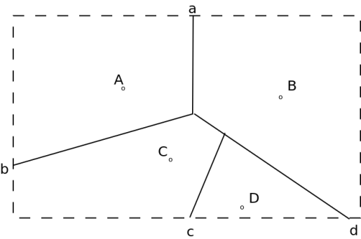
For instance, let’s consider 4 points on which we run the generateVoronoi, we have those edges:

(the dashed lines represent the borders of the image and are not edges returned by generateVoronoi)

The edges associated to each region don’t form a polygon. To close the polygons, we are going to do the following for each region:

• extract the vertices from the edges
• sort the vertices by the angle they form with the x-axis by using the atan2 function (clockwise)
• add missing corner vertices

To find which corner vertex need to be added, we check the position of each vertex and the next one (clockwise):

• if one vertex is on the border and the next vertex is on the next border(clockwise), add a corner vertex
• if one vertex is on the border and the next vertex is on the opposite border, add two corner vertices

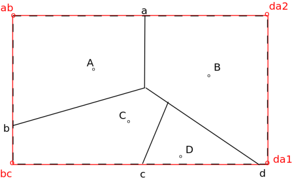
So in order to complete the region A, we have to add a vertex at the top-corner (ab). For the region B, we have to add two vertex corners: on the bottom-right(da1) and at the top-right corner(da2). For the region C, we have to add a vertex at the bottom-left corner(bc).

The code to close the polygons and draw them on the map is the following:

    // will hold the polygon points for each region
    val voronoiCellByGroup = new Array[mutable.Buffer[(Double, Double)]](clusterCount)

    for (group <- 0 until clusterCount) {
      val points = edgeBySite(group) flatMap { edge => Array((edge.x1, edge.y1), (edge.x2, edge.y2))}

      val centerX = clusterCenters(group)(0)
      val centerY = clusterCenters(group)(1)

      // sort the points by ascending angle (between the x-axis and the point)
      val sortedPoints = points.sortBy {
        case (px, py) =>
          math.atan2(py - centerY, -px + centerX)
      }

      val completedPoints = mutable.Buffer.empty[(Double, Double)]

      // because of the image border, we have to add the corner points
      for (i <- 0 until sortedPoints.size) {
        val point = sortedPoints(i)
        val nextPoint = sortedPoints((i + 1) % sortedPoints.size)
        completedPoints += point

        (point._1, point._2, nextPoint._1, nextPoint._2) match {
          case (_, -90d, -180d, _) => // missing bottom-left corner
            completedPoints += ((-180d, -90d))
          case (180d, _, _, -90d) => // missing bottom-right corner
            completedPoints += ((180d, -90d))
          case (_, 90d, 180d, _) => // missing top-left corner
            completedPoints += ((180d, 90d))
          case (-180d, _, _, 90d) => // missing top-right corner
            completedPoints += ((-180d, 90d))
          case (_, -90d, _, 90d) => // missing bottom-left corner and top-left corners
            completedPoints += ((-180d, -90d))
            completedPoints += ((-180d, 90d))
          case (-180d, _, 180d, _) => // missing top-left corner and top-right corners
            completedPoints += ((-180d, 90d))
            completedPoints += ((180d, 90d))
          case (_, 90d, _, -90d) => // missing top-right corner and bottom-right corners
            completedPoints += ((180d, 90d))
            completedPoints += ((180d, -90d))
          case (180d, _, -180d, _) => // missing bottom-right corner and bottom-left corners
            completedPoints += ((180d, -90d))
            completedPoints += ((-180d, -90d))
          case _ =>
        }
      }

      voronoiCellByGroup(group) = completedPoints
    }

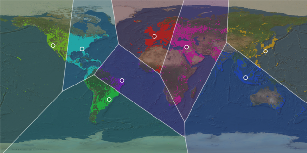
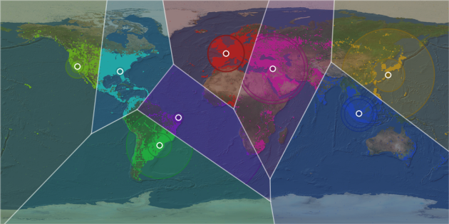
The resulting image with the voronoi cells is now looking like this:

 

Percentile circles

To show the concentration of tweets around the center, we are going to draw two circles around each cluster center:

• 50 percentile circle: this circle contains 50% of the tweets closest to the center
• 90 percentile circle: this circle contains 90% of the tweets closest to the center

To compute the percentile, we sort the tweets in each region by their distance to the cluster center. The radius of the 50 percentile circle is the distance of the tweet at the middle of the sorted list. For the radius of the 90 percentile circle is the one located at the following position: (0.9 * number_of_tweets).

    for ((group, tweets) <- tweetsByGoup) {
      val clusterCenter = clusterCenters(group)

      val distances = tweets
        .map {
        case coordinates: Array[Double] =>
          val dx = clusterCenter(0) - coordinates(0)
          val dy = clusterCenter(1) - coordinates(1
          Math.sqrt(dx * dx + dy * dy)
        }
        .toList
      distances.sortBy(_.toDouble)

      val tweetCount = tweets.size
      val percentile50 = distances((tweetCount * 0.50d).toInt)
      val percentile90 = distances((tweetCount * 0.90d).toInt)

      val color = groupColors(group).brighter()
      val (x, y) = toImageCoordinates(clusterCenters(group)(0), clusterCenters(group)(1), imageWidth, imageHeight)

      // draw circle for percentiles
      val radius50 = (percentile50 * imageWidth / 180).toInt
      val radius90 = (percentile90 * imageWidth / 180).toInt

      val polygon = new Polygon()
      val points = voronoiCellByGroup(group)
      for((px, py) <- points) {
        val (imgX, imgY) = toImageCoordinates(px, py, imageWidth, imageHeight)
        polygon.addPoint(imgX, imgY)
      }
      graphics.clip(polygon)

      val alphaColor = new Color(color.getRed, color.getGreen, color.getBlue, 40)
      graphics.setColor(alphaColor)
      graphics.fillOval(x - radius50, y - radius50, radius50 * 2, radius50 * 2)
      graphics.fillOval(x - radius90, y - radius90, radius90 * 2, radius90 * 2)

      val borderColor = new Color(color.getRed, color.getGreen, color.getBlue, 200).darker()
      graphics.setColor(borderColor)
      graphics.drawOval(x - radius50, y - radius50, radius50 * 2, radius50 * 2)
      graphics.drawOval(x - radius90, y - radius90, radius90 * 2, radius90 * 2)

      graphics.setClip(0, 0, imageWidth, imageHeight)
    }

With those circles, we can see that most of the tweets in the America West Coast Cluster are all grouped very closely to the center. This is not the case for the tweets in the East Asia cluster which are more loosely located.

Draw tweet count

Finally, we can show the number of tweets in each region.

    graphics.setColor(Color.WHITE)
    val numberFormat = NumberFormat.getNumberInstance(Locale.US)
    val font = new Font(Font.SANS_SERIF, Font.BOLD, 18)
    graphics.setFont(font)
    for ((group, tweets) <- tweetsByGoup) {
      val tweetCount = numberFormat.format(tweets.size)
      val bound = font.getStringBounds(tweetCount, graphics.getFontRenderContext)
      val (x, y) = toImageCoordinates(clusterCenters(group)(0), clusterCenters(group)(1), imageWidth, imageHeight)
      // draw text shadow
      graphics.setColor(Color.BLACK)
      graphics.drawString(tweetCount, (x - bound.getWidth / 2).toInt + 1, (y + bound.getHeight + 10).toInt + 1)
      // draw text
      graphics.setColor(Color.WHITE)
      graphics.drawString(tweetCount, (x - bound.getWidth / 2).toInt, (y + bound.getHeight + 10).toInt)
    }

To run the whole program:

sbt "run-main com.chimpler.example.kmeans.KMeansApp tweets.csv tweets.png

Then open the file tweets.png with your favorite image viewer.

Conclusion

We have seen in this post how to listen to tweet streams and then use spark to cluster the tweets by location. We described some techniques to visualize the clusters on a map by dividing the map into voronoi cells and show the concentration of tweets using percentile circles around the cluster centers.

The k-means can be used for other applications such as clustering news based on their textual content, it will be the subject of another post.